Homework 8
ARIMA
Getting started
Start with the following steps:
Go to our RStudio Server at http://turing.cornellcollege.edu:8787/
Open the respective file from the shared STA364_inst_files folder mentioned above. It will be named something like hw-0X_LAST_NAME.qmd.
Then you need to save your copy. Click File -> Save as -> Navigate to the folder
STA364_Projects(that we share) -> Change the “LAST_NAME part of the file name to your last name -> Save.Update the top of the document, called the
YAML,with your name.
Exercises
Problems
Question 1 (fpp9_1)
The following plots show the autocorrleations for 36 random numbers, 360 random numbers and 1,000 random numbers.
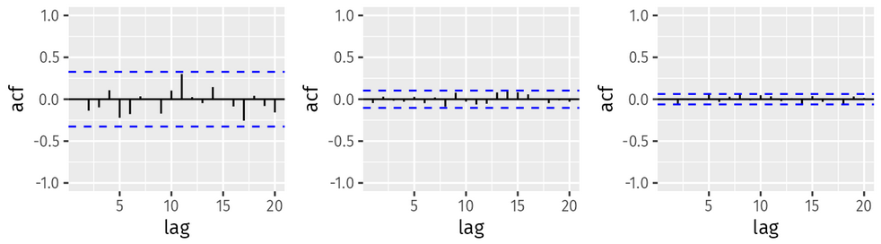
Figure 1: Left: ACF for a white noise series of 36 numbers. Middle: ACF for a white noise series of 360 numbers. Right: ACF for a white noise series of 1,000 numbers.
Explain the differences among these figures. Do they all indicate that the data are white noise?
Why are the critical values at different distances from the mean of zero? Why are the autocorrelations different in each figure when they each refer to white noise?
Question 2 (ffp9_2)
A classic example of a non-stationary series are stock prices. Plot the daily closing prices for Amazon stock (contained in gafa_stock), along with the ACF and PACF. Explain how each plot shows that the series is non-stationary and should be differenced.
Question 3 (ffp9_3)
For the following series, find an appropriate Box-Cox transformation and order of differencing in order to obtain stationary data.
Turkish GDP from global_economy.
Accommodation takings in the state of Tasmania from aus_accommodation.
Monthly sales from souvenirs.
Question 4 (fpp9_7)
Consider aus_airpassengers, the total number of passengers (in millions) from Australian air carriers for the period 1970-2011.
Use ARIMA() to find an appropriate ARIMA model. What model was selected. Check that the residuals look like white noise. Plot forecasts for the next 10 periods.
Plot forecasts from an ARIMA(0,1,0) model with drift and compare these to part a.
Plot forecasts from an ARIMA(2,1,2) model with drift and compare these to parts a and b. Remove the constant and see what happens.
ARIMA(Passengers ~ 1 + pdq(2,1,2)has the constant and,
ARIMA(Passengers ~ 0 + pdq(2,1,2)does not have a constant.
- Plot forecasts from an ARIMA(0,2,1) model with a constant. What happens?
Question 5 (fpp9_11)
Choose one of the following seasonal time series: the Australian production of electricity, cement, or gas (from aus_production).
Do the data need transforming? If so, find a suitable transformation.
Are the data stationary? If not, find an appropriate differencing which yields stationary data.
Identify a couple of ARIMA models that might be useful in describing the time series. Which of your models is the best according to their AIC values?
Estimate the parameters of your best model and do diagnostic testing on the residuals. Do the residuals resemble white noise? If not, try to find another ARIMA model which fits better.
Forecast the next 24 months of data using your preferred model.
Compare the forecasts obtained using
ETS().
Submission
When you are finished with your homework, be sure to Render the final document. Once rendered, you can download your file by:
- Finding the .html file in your File pane of RStudio (on the bottom right of the screen)
- Click the check box next to the file
- Click the blue gear above and then click “Export” to download
- Submit your final HTML document to the respective assignment on Moodle